Breadth First Search Algorithm: Explained with Examples, Code and Video
The series of articles on algorithms have previously been based on data structures and algorithms as it is taught at university.
Now we move into more advanced algorithms in the area of artificial intelligence that are applied to solve problems.
Visiting each part of a tree or graph, called nodes, is called traversal. So to visit a node, or to identify a path in the tree or graph we can use an algorithm to traverse it.
We have seen the basics of data structures like queues and stacks; now it’s time to use them when we implement algorithms for tree or graph traversal.
The initial algorithms to learn are the breadth-first search and the depth-first search (the bfs and dfs algorithms).
In this, the first of two articles on these graph traversal algorithms, we look at the breadth-first search algorithm.
Understanding Breadth First Search

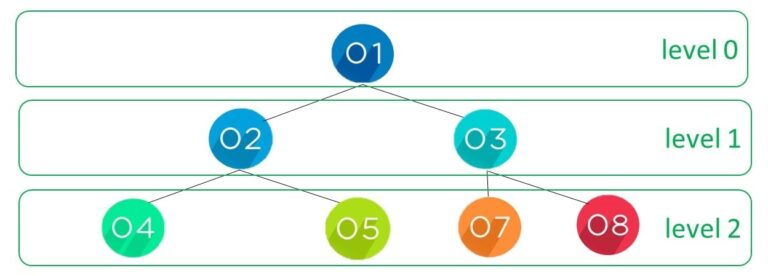
Figure 1. Tree traversal using the bfs algorithm (bfs traversal)
Figure 1 displays a tree with seven elements, also called nodes. When we look for these elements, there are different paths that we can take.
We start off at the root node, which we can see is an element with the value one. In the breadth-first search we look at each node from left to right on each level in order.
In this example, we start with the root node at level zero, then the next level one has elements two and three, and finally, at level two, we have elements four, five, seven, and eight.

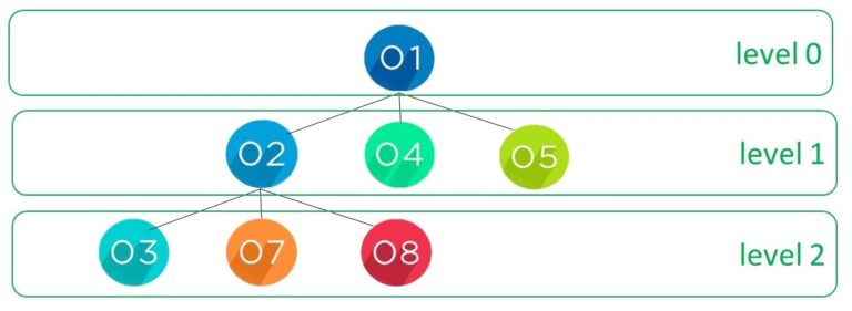
Figure 2. Example of Breadth-first traversal
In Figure 2 we have another example of tree traversal using the bfs algorithm. Visiting each node we start with level zero with the element with one, then level one we have elements two, four, and five. Finally, at level two, we have elements three, seven, and eight.
Implementation of BFS
To implement the BFS algorithm we use a queue. To explain this we use the following example and explain each stage of putting in and taking out nodes from the queue such that we can visit each node i.e. traverse the tree. Let’s see the example tree:

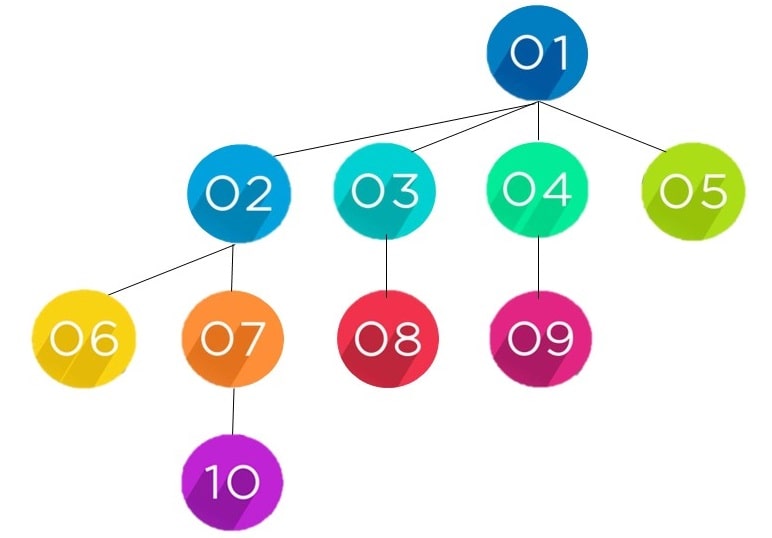
Figure 3. Example of a tree used to explain breadth-first search
To demonstrate the order we visit each node the example tree seen in Figure 2, we show the nodes in both the queue and the list used to store the nodes that have already been visited.

The queue initially starts with the root node. We push the root node, 1, into the queue. The tree, like a family tree, has nodes and children nodes that are seen to be connected to the parent node by the lines seen in Figure 3.
As there is only one root node this will immediately be removed, or popped, from the queue, but not before the ‘children’ of this node are located. These child nodes are then put into the queue in left-to-right order.

From the node 1 we have the children nodes 2, 3, 4 and 5. We put the 2, 3, 4, and 5 elements into the queue and then pop the one because we’ve already visited it.
We keep the visited nodes in a list so we don’t duplicate them in the queue. This is especially important for graphs.

We can see from the tree in the example that the 2 node has two children 6 and 7. We enter the 6 and 7 elements at the end of the queue and pop 2 into the list of visited nodes.

Node 3 has the child node 8 therefore 8 is entered into the queue and 3 is popped.

Node 4 has the child node 9 therefore 9 is entered into the queue and 4 is popped.

Nodes 5 and 6 have no children and are removed from the list and entered into the visited list..

Node 7 has the child node 10 therefore 10 is entered into the queue and 7 goes to the visited list.

The final three nodes of 8, 9 and 10 all have no children therefore they are placed into the visited list which is now complete.
We can see the order that the nodes were visited, 1, 2, 3, 4, 5, 6, 7, 8, 9, and 10. The breadth first search BFS algorithm has traversed the tree.
Video Tutorial
If you would like to see all these example of the bfs algorithm explained then watch this video tutorial, enjoy!
BFS Algorithm Implementation in Python
Here is the python code for implementing breadth-first search using the deque from the collections module.
from collections import dequeInitially we create the tree using a dictionary with the parent node as the key and the chidren nodes in a list.
tree = {
    1: [2, 3, 4, 5],
    2: [6, 7],
    3: [8],
    4: [9],
    5: [],
    6: [],
    7: [10],
    8: [],
    9: [],
    10: [1]
}
We use the deque, starting with the root node. We pop from the beginning and append the children nodes to the queue at the end, if they haven’t been visited before and are not already in the queue.
def breadth_first_search(tree, start):
    queue = deque([start])
    visited = []

    while queue:
        node = queue.popleft()
        visited.append(node)

        for child in tree[node]:
            if child not in visited and child not in queue:
                queue.append(child)

    return visited
Finally we call the python function with the tree and the root node which in this example is 1.
result = breadth_first_search(tree, 1)
print(result)
To see the example in the final code with each stage before and after the nodes are entered and popped from the queue we have added two print statements.
from collections import deque

tree = {
    1: [2, 3, 4, 5],
    2: [6, 7],
    3: [8],
    4: [9],
    5: [],
    6: [],
    7: [10],
    8: [],
    9: [],
    10: [1]
}
def breadth_first_search(tree, start):
    queue = deque([start])
    visited = []

    while queue:
        print("before ", queue)
        node = queue.popleft()
        visited.append(node)

        for child in tree[node]:
            if child not in visited and child not in queue:
                queue.append(child)
        print("after ", queue)
    return visited

result = breadth_first_search(tree, 1)
print(result)
Here is the output:
before  deque([1])
after  deque([2, 3, 4, 5])
before  deque([2, 3, 4, 5])
after  deque([3, 4, 5, 6, 7])
before  deque([3, 4, 5, 6, 7])
after  deque([4, 5, 6, 7, 8])
before  deque([4, 5, 6, 7, 8])
after  deque([5, 6, 7, 8, 9])
before  deque([5, 6, 7, 8, 9])
after  deque([6, 7, 8, 9])
before  deque([6, 7, 8, 9])
after  deque([7, 8, 9])
before  deque([7, 8, 9])
after  deque([8, 9, 10])
before  deque([8, 9, 10])
after  deque([9, 10])
before  deque([9, 10])
after  deque([10])
before  deque([10])
after  deque([])
[1, 2, 3, 4, 5, 6, 7, 8, 9, 10]
Graph Traversal using Breadth First Search
We can also use breadth first search for graphs using the same principle.
A circles with a number represents a node which in graphs is also called a vertex.The lines attaching these nodes or vertices are called edges.
Directed graphs have arrows as edges and undirected graphs have lines as edges.

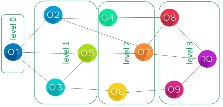
Figure 4. Example of breadth-first traversal of a graph
The start node is on level-zero to the far left with the value 1. This element 1 is connected to 2, 5, and 3 at level one.
The element with the value 2 connects to 4 and 7. element valued 5 also goes to 7, but we only visit an element once.
3 connects to 6, so, at level two, we have elements 4, 7, and 6in that order.
Now, 4 was first, so this initially goes to 8. Then we have 7, connected to 10, and 6, which goes to 9. In the final level 3, we have elements 8, 10 , and 9.
The BFS graph algorithm uses the same process to traverse the graph as the algorithm traverses the tree.
The graph traversal uses the same python code seen in the tree example above.
    g = Graph()
    g.addEdge(1, 2)
    g.addEdge(1, 5)
    g.addEdge(1, 3)
    g.addEdge(2, 4)
    g.addEdge(2, 7)
    g.addEdge(3, 5)
    g.addEdge(3, 6)
    g.addEdge(4, 8)
    g.addEdge(5, 7)
    g.addEdge(6, 9)
    g.addEdge(7, 10)
    g.addEdge(8, 10)
    g.addEdge(9, 10)
Figure 5. A graph is represented by an adjacency list of edges. This code is seen in the next article on depth first search.
There are no unvisited nodes, and the process can be used on graphs with a high number of edges
In practice this could represent a network, or a minimum spanning tree. Also it can be used to find the shortest path by visiting the adjacent nodes, applying the algorithm on an unweighted graph.
Time Complexity Question
Q. Will the time complexity of BFS be O(V) considering we only have to traverse the vertices in the adjacency list?
A. The graph is represented by a list of associated nodes, called vertices, this is called the adjacency list.
Each pair of nodes or vertices are joined in the graph by the edges. In breadth-first search (BFS), the time complexity is s O(V + E), where V is the number of vertices and E is the number of edges in the graph.
This is because it visits each node and its adjacent edges once during the traversal.

